Three saved measurements tell us where the bass is strong, where the response dips, what changes between runs, and what remains after the initial arrival. The most useful discovery is that these are different questions.
Best file.mdat · 3 saved sweeps · approximately 10–150 Hz · saved labels dated September 7–8, 2015 · report prepared October 8, 2026
A repeatable broad response, with an unstable fine detail.
Stored measurements
33 & 61 Hz
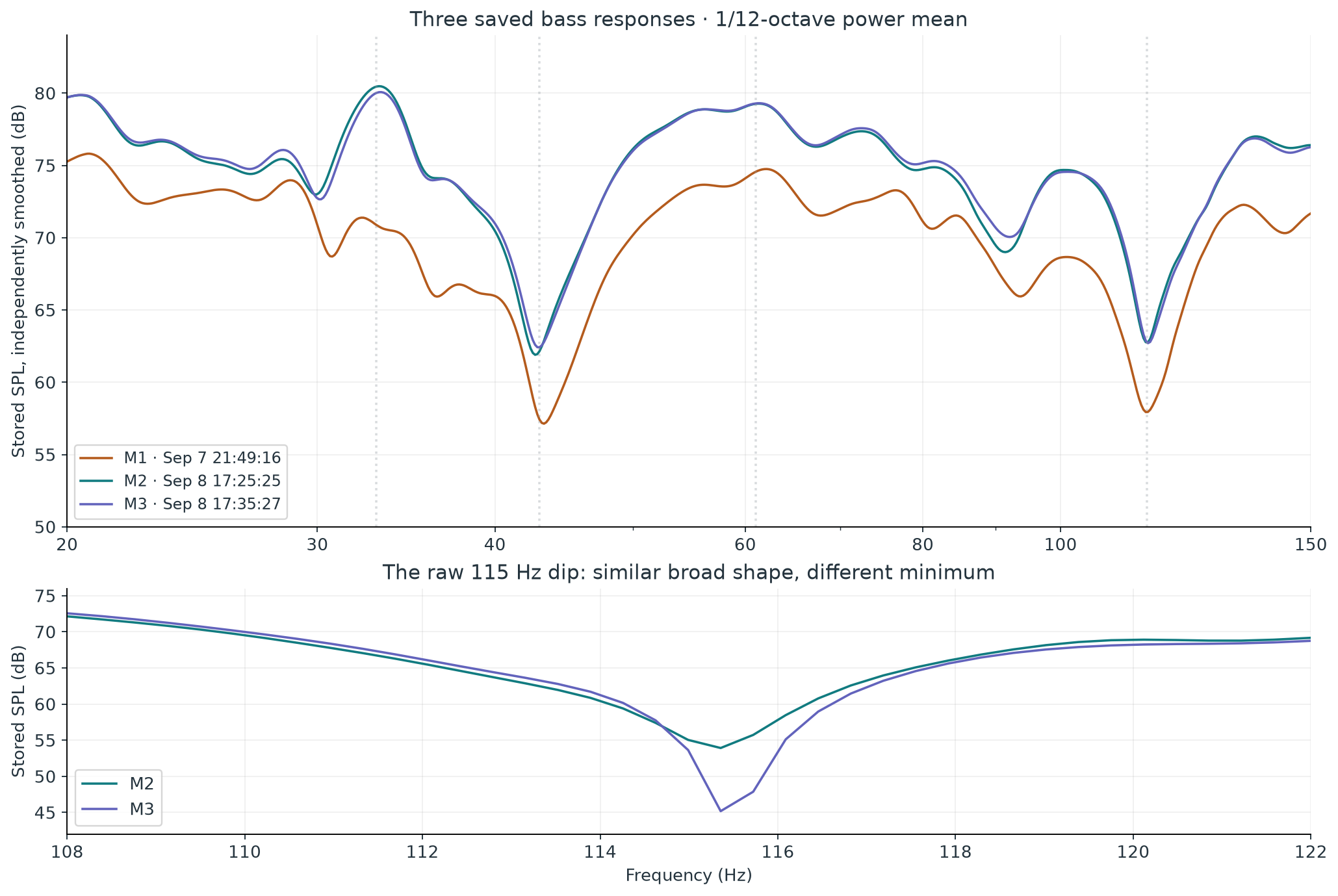
Prominent peaks in M2 and M3. Dips appear around 43 Hz, 92 Hz, and 115 Hz.
Derived comparison
0.67 dB
RMS M2–M3 difference after removing their median level offset over 20–150 Hz. A descriptive metric, not an uncertainty bound.
Stored measurements
8.74 dB
Difference at the raw 115.36 Hz minimum between those same two runs. Smoothing largely hides it.
These are archived measurements of the owner's subwoofer. That source identification comes from your correction; the subwoofer model, crossover settings, placement, and whether the main speakers were active during the sweeps remain unconfirmed. The measurements describe the subwoofer's response through the room and measurement chain. They cannot establish its present-day condition or rate the whole speaker system.
High confidence · observation
Three response records, one meter calibration.
Each saved record contains a different SPL response and impulse response. All three embed the same RadioShack-33-2055-4050-CS.cal curve. There is no fourth saved record labeled as a flat meter reference. A calibration curve may have been displayed beside the measurements, but that cannot be identified from the file alone.
High confidence · calculated
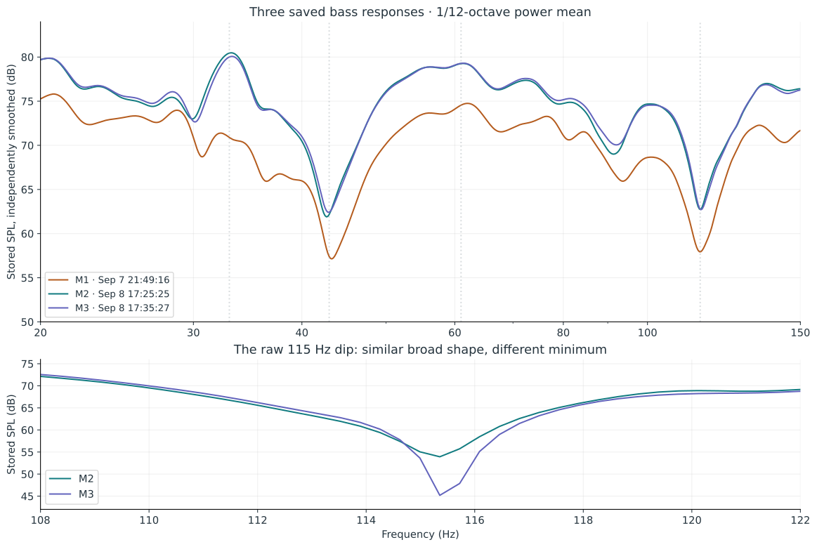
Similar curves can conceal a changing null.
M2 and M3 were saved about 10 minutes 2 seconds apart. Their broad response is strongly correlated, yet the minimum around 115 Hz falls from 53.92 to 45.18 dB. This makes a controlled repeat and a small position test more valuable than an immediate boost at that frequency.
Moderate confidence · interpretation
The loudest peak is not the longest tail.
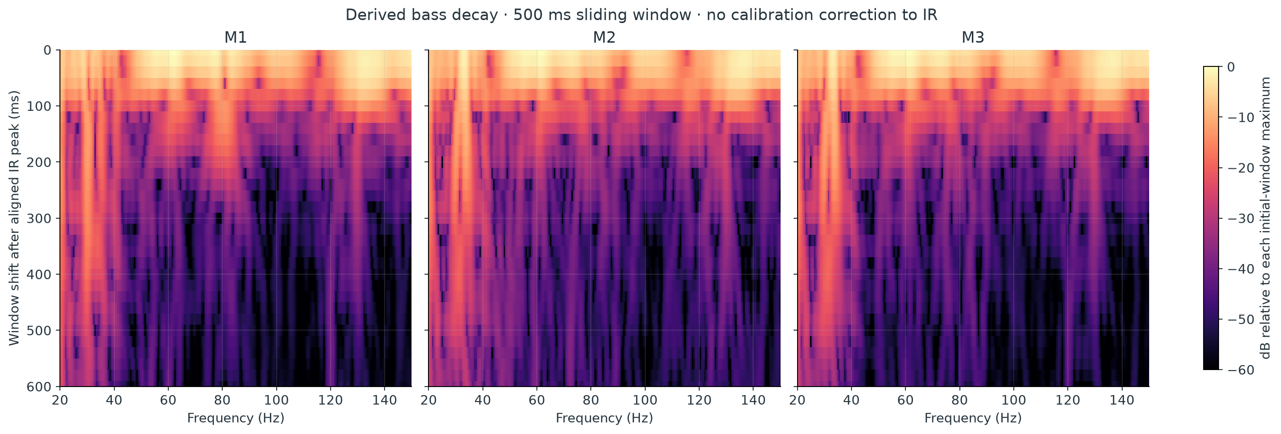
Windowed spectra show substantially more lingering low-frequency energy near 20 Hz and 30–35 Hz than near 61 Hz. Window-length checks preserve that ranking, although exact late-spectrum peak locations move. The data supports a low-bass persistence finding; it does not identify a specific room mode.
Unresolved · cause
The dips have several possible explanations.
Cancellation from boundaries, interactions between sources, existing filters, and measurement conditions remain plausible. Without source-isolated measurements, room dimensions, and documented positions, none can be selected as the physical cause.
02 · Frequency response
Where the bass rises and falls.
Start with the 1/12-octave view for the broad shape. Switch to the stored unsmoothed data to inspect narrow features. The source spacing is 0.36621 Hz; interpolation adds readable positions between samples but does not increase measurement resolution.
The scan follows recorded curves; it is not an audio playback or an animation of waves in the room. “Subtract median” is a derived shape comparison, using a uniform log-frequency grid over 20–150 Hz. Click a legend entry to show or hide a response.
Feature
M2
M3
Meaning
Peak near 33 Hz
33.15 Hz · 80.48 dB
33.27 Hz · 80.07 dB
Stable broad feature in the two later runs.
Dip near 43 Hz
42.69 Hz · 61.90 dB
42.99 Hz · 62.42 dB
Large and persistent under this smoothing.
Peak near 61 Hz
61.24 Hz · 79.27 dB
61.24 Hz · 79.30 dB
Very similar level and position.
Dip near 92 Hz
91.43 Hz · 69.00 dB
92.10 Hz · 70.05 dB
A smaller trough that also changes slightly.
Dip near 115 Hz
115.20 Hz · 62.75 dB
115.20 Hz · 62.70 dB
These smoothed values conceal different raw minima.
Feature values above are calculated from the independent 1/12-octave power-mean curve, not claimed to be exact REW graph readings. They are feature positions on that derived grid, not uncertainty estimates. M3's 5th–95th percentile span is 13.84 dB under the same processing. This describes unevenness in these bass data; it is not an audibility score or a speaker-quality rating.
03 · Relationships between measurements
Separate a level change from a shape change.
M2 and M3: closely matched overall
115 Hz: a magnifying glass
The median M3–M2 offset is only +0.066 dB. After subtracting it, the log-frequency RMS difference is 0.671 dB and the response correlation is 0.989. These are similarities between stored runs. The notes do not prove that equipment, position, background noise, or settings were held constant.
At 115.36 Hz the raw difference is −8.74 dB. In M3 the minimum is approximately 23.90 dB below the mean of the interpolated 110 and 120 Hz shoulders. That is a defined local depth, not a deviation from a verified target.
A useful distinction: the broad dip is repeatable; its deepest sample is less stable. The low residual level, interference, and small configuration or position changes could all matter. There is no independently verified noise-floor trace here that establishes which explanation applies.
M1 sits lower than M2 by a median 4.92 dB over the same comparison band. The saved SPL calibration offset also changes by 1.699 dB, and the saved EQ target changes from 71.7 to 75.0 dB. Even after removing the median level shift, M1–M2 retains 2.13 dB RMS shape difference. The file does not support calling this an improvement caused by a known adjustment.
04 · Frequency and time together
Watch the energy that remains.
A frequency-response peak tells us about level. A decay slice asks what frequency content remains in a later portion of the impulse response. Here the slow low-bass tail is more interesting than the prominent 61 Hz peak.
Grey: the initial window. Colored: the selected later window. Each spectrum is calculated from the saved IR, with a 100 ms rise before the selected time and a 400 ms right window. The time label is a window shift, not a sharply isolated instant. All slices use a fixed reference: that run's initial-window maximum over 20–150 Hz.
M1
M2
M3
At a 400 ms window shift
M2
M3
20 Hz · change from its own initial slice
−10.6 dB
−10.7 dB
33 Hz · change from its own initial slice
−22.6 dB
−20.2 dB
61 Hz · change from its own initial slice
−56.0 dB
−44.6 dB
These figures are windowed spectral retention, not RT60 values. Values near the late noise floor are less precise, particularly the very low 61 Hz residuals. Using right windows of 250, 400, and 600 ms preserves the much slower 20 Hz tail relative to 61 Hz. It does not preserve every small late peak or every detailed attenuation value.
Interpretation Resonant storage, source or filter behavior, and the limited sweep bandwidth could contribute to the low-bass persistence. A stronger room-mode conclusion would require geometry and position tests. REW's explanation of waterfalls also emphasizes the tradeoff between frequency resolution and time smearing. Source: REW waterfall methodology
05 · Impulse response and remaining energy
A short initial arrival, followed by a bass tail.
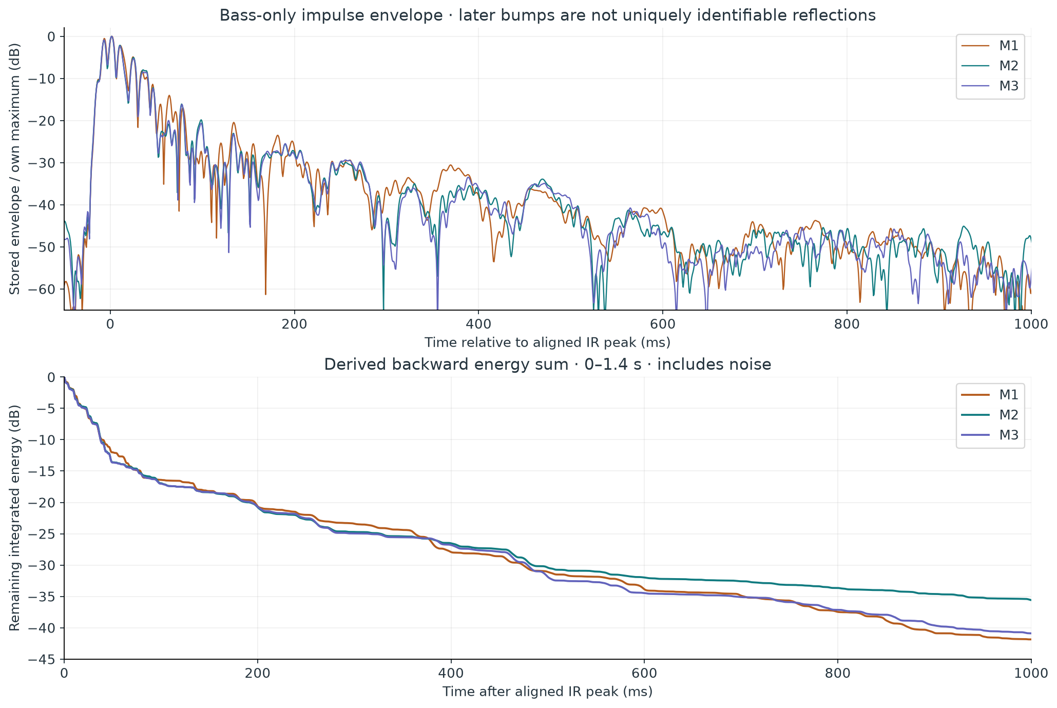
The envelope is stored data normalized to each run's own maximum. The absolute IR peaks are aligned at t = 0 in all three records. The envelope maxima follow by approximately 1.3–2.0 ms.
In a simple backward sum of squared IR samples from 0 to 1.4 seconds, remaining energy reaches −20 dB at 191–197 ms and −30 dB at 475–485 ms. The agreement is useful even though fine spectral details differ. This derived sum includes noise and uses the finite retained record; later crossings are more sensitive to those choices.
Do not turn these bumps into a map of the room. The retained IR has an effective sample rate of 1,500 Hz and a measurement bandwidth ending near 150 Hz. Its broad lobes include bass oscillation and band-limiting effects. It cannot uniquely identify an early wall reflection, tweeter alignment, or a physical travel distance.
The saved acquisition sample-rate field is zero. The 1,500 Hz rate comes from the IR sample interval of 0.000666667 seconds, and is the rate of this retained IR—not evidence of the soundcard's original recording rate. The leftAsTimingRef flag is false and the stored measurement delay is zero. Original-peak-time fields differ between runs; with no documented common timing reference they should not be converted into source distances.
The file also contains legacy decay fits
These saved fit values are reproduced for transparency, not adopted as a room-wide reverberation estimate. Their IR is bass-limited, and the stored T20 fit coefficients have magnitudes below 0.99.
Run
Stored EDT (s)
Stored T20 (s)
T20 fit r
Stored Topt (s)
M1
0.282
1.047
-0.938
1.631
M2
0.289
0.923
-0.929
1.306
M3
0.281
0.989
-0.921
1.648
REW explains that low-frequency RT60 is generally not meaningful in small domestic rooms dominated by modes, and recommends decay or spectral views for this region. The −20 dB energy crossing above is an elapsed crossing time, whereas a T20 fit extrapolates a fitted slope to 60 dB; they are different quantities. Source: REW RT60 definitions and limits
06 · Phase and group delay
Timing behavior adds evidence, but not a unique diagnosis.
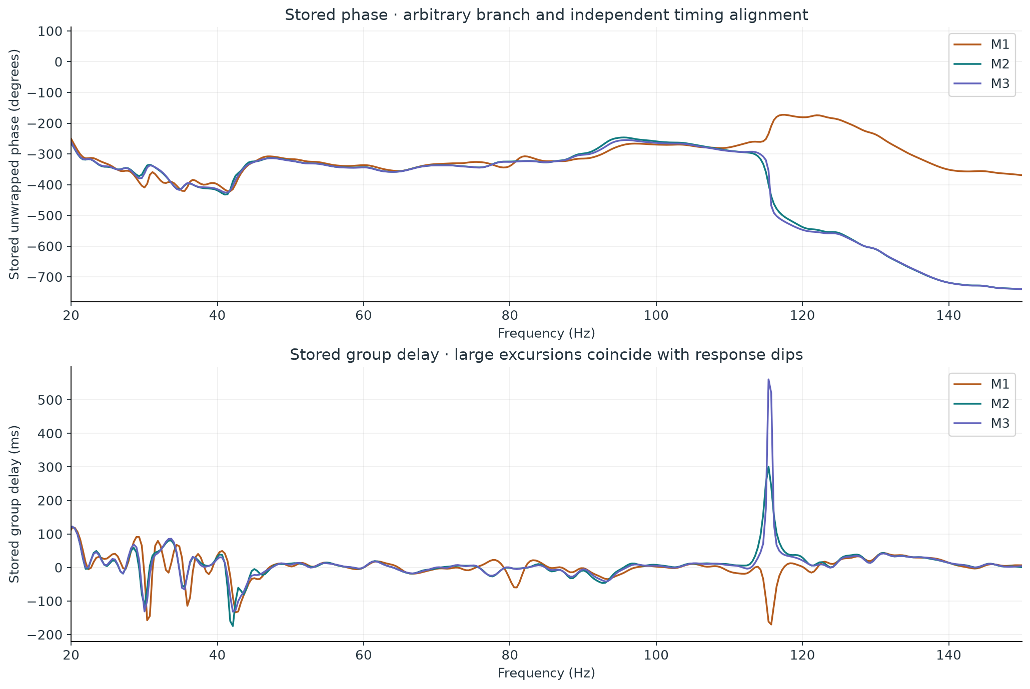
Stored unwrapped phase
Stored group delay
Group delay is calculated from phase slope. The strongest excursions coincide with response dips, including the 115 Hz region. A steep phase change where very little signal remains is a reason to inspect magnitude and timing together; it is not sufficient evidence that a component is defective. Negative group-delay values here do not mean sound traveled backwards in time.
Unwrapped phase has an arbitrary whole-turn branch, and each IR has been aligned independently. There are no identified main-speaker measurements sharing a documented timing reference with these subwoofer runs, so they cannot support a reliable main-plus-subwoofer complex sum, optimum relative delay, or polarity prescription. The saved 80 Hz speaker-cutoff field may be a target/setup parameter; it does not prove that the actual system crossover was 80 Hz. Source: REW group delay and timing reference
07 · What the meter contributes
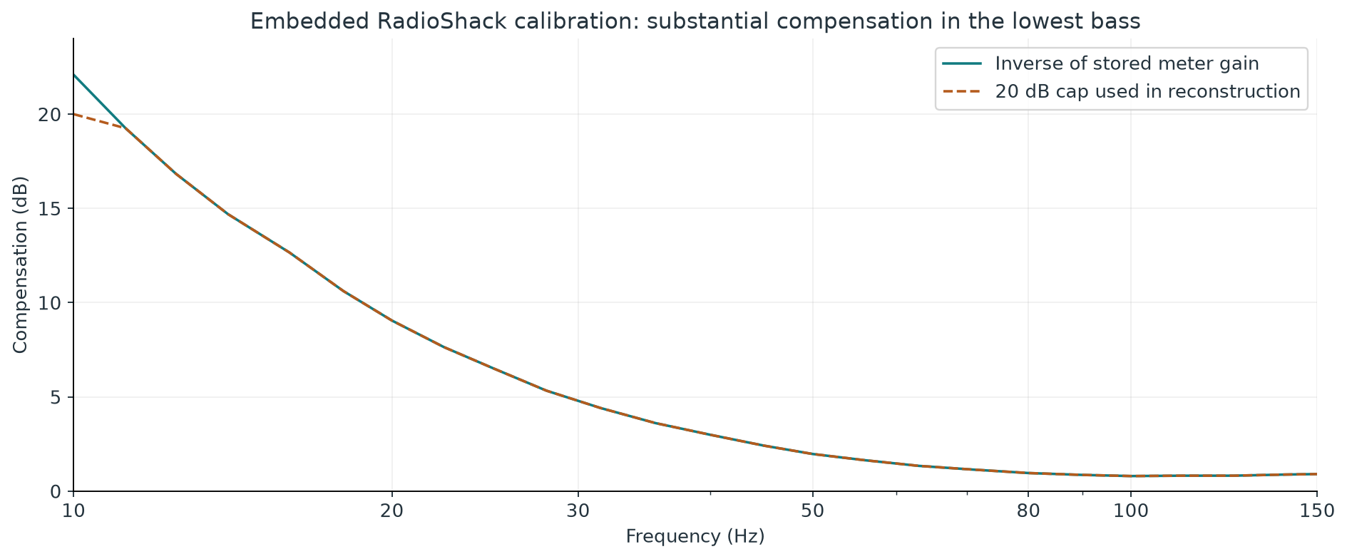
The lowest bass depends heavily on compensation.
The embedded meter gain is −9.05 dB at 20 Hz, −4.41 dB at 31.5 Hz, −1.97 dB at 50 Hz, and −0.96 dB at 80 Hz. Removing that stored meter response adds the corresponding positive compensation to the raw transfer magnitude. At 10 Hz the table calls for 22.09 dB, but the stored calibration-limit flag is active; a 20 dB cap reproduces the saved magnitude convention.
All three stored SPL curves already include the same calibration response. It must not be applied a second time. The calibration file contains zero phase values, so it supplies no frequency-dependent meter-phase correction. The inverse-C flag is also selected; the embedded gain table spans the measured band, so a second C-weighting compensation is not added here. Source: REW calibration-file conventions
Practical implication The file documents which correction was used; it does not establish that it accurately calibrated this individual meter. The 10–20 Hz region is especially dependent on instrument response and has larger run differences. A modern individually calibrated microphone would provide a valuable independent check before attempting a low-bass correction.
08 · Distortion: data present, interpretation constrained
The file cannot establish the subwoofer's distortion limits.
Each record includes 11 legacy spectral rows at 376 frequencies, from 10 to approximately 149.93 Hz. They are retained without alteration in the downloadable data as stored_row_0 through stored_row_10. The legacy row labeling, noise-floor treatment, and calibration treatment have not been validated against an authoritative V5.12 schema. This report therefore does not assign a definitive THD percentage or diagnose a driver from those arrays.
Bandwidth is a separate limitation: the saved fundamental-response range does not independently establish the valid range of every harmonic row. If 150 Hz was also the excitation sweep's upper limit, second-harmonic results above approximately 75 Hz and third-harmonic results above approximately 50 Hz would require output beyond that sweep limit. The measuring chain can also contribute distortion. A documented, wider-band measurement at several modest levels with a suitable microphone would resolve these limitations. Source: REW distortion bandwidth and measurement-chain limitations
09 · A correction thought experiment
Try small cuts in the model; investigate deep dips physically.
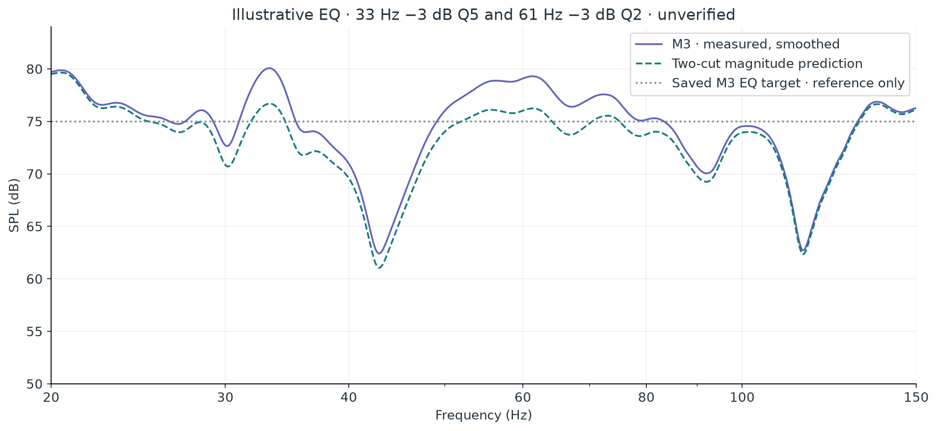
The two later measurements show similar peaks around 33 and 61 Hz. A conservative illustrative model applies 33 Hz / −3 dB / Q 5 and 61 Hz / −3 dB / Q 2 to M3. This is a deliberately limited scenario, not an optimized filter prescription.
Simulation · not applied
The model uses standard digital peaking filters at an assumed 48 kHz calculation rate. It contains no positive gain; no boost headroom is demanded by these filters. Their combined maximum response over the full digital band is approximately 0 dB. The saved 75 dB target is displayed only as a reference—there is no evidence that a flat line is the owner's preferred or appropriate house curve.
The prediction applies no boost to the deep 43 and 115 Hz dips. It shows how the magnitude curve would change under this filter model at the measured position. It does not demonstrate an audible improvement, reduced room decay, better seating-area consistency, or compatibility with a specific hardware filter implementation. The file's saved DSP1124P filter slots are all NONE with zero gain, despite notes saying “filters engaged”; existing external filter settings cannot be recovered from those slots.
For a cancellation, extra drive can expend headroom without reliably filling the hole, and the result can change at another seat. Multi-position verification should precede a real filter decision. Source: REW's limits of EQ
10 · The most valuable next measurements
Five experiments, ordered by information value.
Establish a documented current subwoofer baseline and repeat it.
Record the subwoofer model and position, whether the mains are active, crossover and EQ settings, meter or microphone, calibration file, level, and microphone position. Take three runs without moving anything. Extend the measured band only where the subwoofer and measurement chain support it.
Discriminates: ordinary repeatability versus the large raw 115 Hz change. If the minimum changes while broad shoulders stay fixed, inspect residual level, noise, and measurement setup before optimizing it.
Move only the microphone by approximately 20 cm.
Measure the original position plus nearby forward/back and left/right positions, with gain and sources fixed. Overlay unsmoothed response and a consistently smoothed shape comparison.
Discriminates: strong spatial cancellation versus a more stable source or filter feature. A shifting/filling 43 or 115 Hz dip strengthens the spatial explanation; it does not by itself identify the responsible boundary.
Measure the subwoofer and mains separately, then together.
For an integration check, measure the sub alone, each main alone, and the intended combinations with one common timing reference, unchanged microphone position, and documented crossover settings. Confirm which sources were active in each run.
Discriminates: a feature already present in the subwoofer response versus cancellation introduced by combining it with the mains. A dip appearing mainly in the combination makes relative phase/delay a stronger candidate.
Check the 20–35 Hz tail with an independent microphone and longer retained IR.
Repeat at the same position and moderate level, retaining enough post-peak data to reach a stable noise region. Compare multiple waterfall windows and nearby positions.
Discriminates: persistent acoustic energy versus effects strongly dependent on meter correction, sweep endpoints, processing, or source filters. Room dimensions become useful if a stable resonance survives those checks.
Compare a modest cut against the current baseline across several positions.
If the 33 or 61 Hz peaks remain stable, test one cut at a time. Match overall playback level when comparing, remeasure the same positions, and inspect both response and decay.
Acceptance: the intended peak reduces without creating a nearby problem or worsening the listening-area spread. Only a remeasurement and listening comparison can turn the preview into a verified improvement.
11 · Presentation choices
What works well for this particular file.
View or animation
Implemented
What it explains
Frequency scan over measured overlays
Yes · play / stop / scrub
Strong and weak bass regions; raw versus smoothed detail.
Response differences and a notch close-up
Yes · interactive plots
Why a small overall difference can include a large local change.
Decaying spectrum playback
Yes · three runs / play / scrub
Energy persistence and the distinction between level and decay.
Impulse-envelope time cursor
Yes · play / stop / scrub
Initial bass arrival, tail, and remaining integrated energy.
Phase, delay, and calibration overlays
Yes · interactive plots
Timing evidence and instrument compensation.
EQ before/predicted view
Yes · explicit simulation toggle
A small-cut thought experiment with no deep-null boosts.
Animated room-mode or reflection geometry
Insufficient geometry and bandwidth
Would require dimensions, positions, and wider-band timing evidence.
Would require position labels, source isolation, common timing, or wider bandwidth.
Animations begin only when requested, stop at the end, and can be scrubbed manually. A reduced-motion preference leaves manual controls available without starting automated motion.
12 · Technical appendix
Enough detail to audit the findings.
Measurement inventory
Record · saved label
Exact saved note
SPL offset
EQ target
M1 Sep 7 21:49:16
Samll front. filters engaged
95.793 dB
71.7 dB
M2 Sep 8 17:25:25
Small filters engaged next day
97.492 dB
75.0 dB
M3 Sep 8 17:35:27
No measurement note saved
97.492 dB
75.0 dB
All records have 384 linearly spaced response points from 9.887695 to 150.146484 Hz, at 0.3662109375 Hz spacing. Each retains 4,096 IR samples from −1.000 to approximately +1.730 seconds. Saved windows use Tukey shapes, with approximately 166.7 ms before and 500 ms after t = 0. The sweep descriptions say 512k log swept sine, 2 sweeps, −12.0 dBFS. Those saved settings are not independently verified acquisition logs.
Labels show September 7 and 8 without a year. The stored epoch timestamps establish 2015. Converted UTC timestamps are supplied in inventory.json; the original label timezone is not asserted. Room dimensions are zero-valued defaults, source positions are absent, and no separate soundcard calibration object is saved.
Extraction and checks
The file is a Java serialization stream. A Python structural reader consumed all 253,488 bytes and decoded its class descriptors, primitive values, arrays, strings, and references without running serialized Java code. A separate Python implementation, javaobj-py3, matched 2,100 field and array checks. No Java runtime or REW application was installed or executed.
A numerical cross-check rebuilt magnitude from the saved windowed IR and embedded calibration. Over 20–150 Hz, the maximum difference from stored SPL was 0.0043 dB. Reconstruction used the file's SPL offset, logarithmic interpolation of its calibration gain, the active 20 dB compensation cap, and a confirmed −3.000 dB magnitude convention offset. This validates the extraction and internal numerical consistency; it does not validate the original meter calibration or the physical measurement setup. Format reference: Oracle object serialization protocol
Independent processing
Response smoothing: interpolate stored dB values onto a 192-points-per-octave grid from 20 Hz to just below 150 Hz; convert to linear power; average 16 adjacent bins; convert back to dB. Edge bins use nearest-value extension. This is a documented independent power mean, not an assertion of identical REW smoothing.
Comparisons: uniform weighting on that log-frequency grid. Remove the median pointwise difference for the reported shape RMS. The response correlation is Pearson correlation of the interpolated dB curves. No uncertainty distribution or controlled repeatability standard is inferred.
Feature detection: peaks and dips on the smoothed grid, prominence at least 2 dB, minimum separation 25 grid points. The deep 115 Hz minima and their 8.74 dB difference use stored raw samples instead.
Decay: saved linear IR without applying meter calibration; 100 ms sine-squared rise before each shift, 300 ms flat right section, then 100 ms cosine-squared fall. FFT zero-padded to 16,384 samples and interpolated to 0.5 Hz plotting intervals over 20–150 Hz. True frequency resolution is governed by the 500 ms window, not zero-padding. Shifts are 20 ms apart; the display covers 0–600 ms. Each run's scale references its own initial-window maximum. Right-window sensitivity was checked at 250, 400, and 600 ms.
Envelope: stored envelope divided by its maximum, displayed as 20 log10 of that ratio. No extra envelope smoothing.
Energy sum: backward sum of squared IR values between 0 and 1.4 seconds, normalized to the energy at 0 seconds. No noise subtraction or reverberation extrapolation. This is a custom bass-energy diagnostic.
EQ: product of two standard peaking biquad responses, 48 kHz model rate, applied to the displayed M3 smoothed magnitude. No source-combination, phase-alignment, spatial, or audibility prediction.
Files and reproducibility
Published alongside this report in data/ and figures/: complete response/phase/group-delay and IR CSV exports, embedded calibration, uninterpreted legacy harmonic rows, derived smoothing and decay matrices, illustrative EQ parameters, inventory, provenance, and shareable PNG/SVG figures. The original REW file is not published; its SHA-256 is listed below.
The interactive report itself is self-contained and works offline. Printing uses the high-resolution figures published alongside it. Keep raw, derived, and simulated files separate when comparing future measurements.